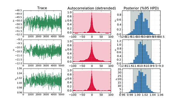
This post presents a few different approaches to model/parameter estimation of a simple mass spring damper system from measured kinematic data. The system is stimulated by a predefined external force record and then the measurements artificially corrupted by noise which is added to the observations.
In order to speed the simulation, and to explore some different approaches, the same dynamic model was implemented in three different ways:
- Pure Python;
- Boost; and
- Cython
First, the pure Python implementation is the most straightforward, but slowest by far. Using Boost has nice features like arrays and access to the odeint library for solving Ordinary Differential Equations. I have also incorporated PyUblas, which provides an (array) interface to Numpy, but this is a legacy thing and not strictly required - it wouldn't require many changes to remove that library if desired. Last, Cython is an easy way of creating C/C++ extensions within the Python source.
The Jupyter notebook explores three main approaches to estimation:
- Linear regression;
- Gradient-based optimisation; and
- Bayesian estimation using sampling
Linear regression is a standard statistical technique and provides a one-step analytical solution (equation error), but is prone to bias in the presence of noise in the independant variables. Gradient-based optimisation is an iterative numerical technique which progressively minimises some cost function - usually the difference in the (simulated) output - but can suffer from local minima. There are many methods which fall under this catagory, two of which are considered here: Powell's method and the Levenberg-Marquardt algorithm. The former is implemented using the SciPy Optimization package and the latter using the Lmfit package. Bayesian estimation is performed using Markov chain Monte Carlo using the PyMC package, with an Adaptive Metropolis step method. In order to improve the sampled estimates, it is common to precede this with another algorithm such as maximum a-posteriori, which puts the coefficients much closer to their true values initially. PyMC employs the SciPy Optimization package to facilitate this.

The full source is here.